Overview
This is a tutorial on the use of xiSEARCH and the xi pipeline for crosslinking mass spectrometry data analysis and structural interpretation. We will walk through how crosslinking MS can be used to answer specific biological questions in structural biology. We will be focusing on a dataset obtained with the photo-crosslinker sulfo-SDA on a purified reconstituted protein complex: the Cullin4 ubiquitin ligase system hijacked by the simian immunodeficiency virus protein Vpr.
SIV suppresses the immune response by recruiting the antiviral restriction factor SAMHD1 to this Cullin4 ligase complex. The key structural questions are how Vpr binds the ligase and which region of SAMHD1 is recruited onto the complex. This work was published as Structural insights into Cullin4-RING ubiquitin ligase remodelling by Vpr from simian immunodeficiency viruses.
A cryo-EM structure of this system could be obtained, but the structure was difficult to interpret. The core reached high resolution, but SAMHD1 was missing from the density, and the system appeared highly flexible, yielding multiple low resolution states in classification (EMD-10612, EMD-10613, EMD-10614). The cryo-EM structure therefore did not fully explain how Vpr recruits SAMHD1 or how SAMHD1 is positioned relative to the ligase.
Crosslinking MS was used to identify the interaction of SAMHD1 with the complex, characterize the flexibility of this Cullin4 ubiquitin ligase assembly, and understand the dynamic position of SAMHD1. In this tutorial, those biological questions provide the reason for the experimental design, the search settings, the FDR choices, and the structural interpretation.
The dataset uses sulfo-SDA crosslinking data from the Cullin4 ubiquitin ligase, SAMHD1, and Vpr system described in the Vpr/Cullin4/SAMHD1 study. The practical goal is not only to generate crosslinks, but to decide which observations are reliable enough to support structural interpretation.
The original tutorial material is maintained in grandrea/crosslinking-ms-tutorial, and the raw mass spectrometry data are available from PRIDE project PXD020453. Background documentation for the search and FDR stages comes from the xiSEARCH and xiFDR documentation.
Who this tutorial is for
This tutorial is intended for users who receive crosslinking MS data from a facility and need to understand what to do next, users who want to reprocess raw-derived files or search outputs, users who need to interpret or leverage crosslinking MS data for structural interpretation, and users who are beginning to optimize crosslinking experiments in-house.
It is not a complete protocol for going from purified protein to raw mass spectrometry data. The experimental sections explain the design logic behind the dataset so that the analysis choices make sense, but they do not replace local wet-lab and MS facility methods.
By the end of the tutorial, you should understand how to set up a database search for crosslinking mass spectrometry. You should also be able to explain why xiFDR-filtered residue pairs are the correct result level for this structural workflow, and why score sliders in visualization tools are for inspection rather than redefining the accepted dataset.
The later modules move from network and sequence-level inspection in xiview to 3D distance checks, ChimeraX/X-MAS visualization, and modeling tools such as DisVis. The emphasis is on turning crosslinks into testable structural hypotheses, not treating every link as a final structural conclusion.
Learning goals
- Explain how crosslinking MS can test a mechanistic hypothesis about Vpr, Cullin4 ligase hijacking, and SAMHD1 recruitment.
- Connect the chemistry of sulfo-SDA to the xiSEARCH configuration used for this dataset.
- Distinguish a scored candidate match from an FDR-controlled crosslink result.
- Explain why error has to be propagated from spectra to peptide pairs, residue pairs, and protein pairs.
- Use xiview to inspect crosslink localization, spectra, condition-specific patterns, and structure-derived distances.
- Separate observations that support a structural model from observations that only motivate a new hypothesis.
How to work through the tutorial
Each module starts with the concept that motivates the action. Read that part first, then perform the boxed instruction or answer the boxed question. The checkboxes are only a local progress aid; they do not store or submit data.
Software and where to get it
Several steps use external tools. Install or open them before the practical session if you want to follow the complete workflow from search to structural interpretation.
| Tool | Where to get it | Used for in this tutorial |
|---|---|---|
| xiSEARCH | Rappsilber Lab xiSEARCH download page | Searching MGF/APL peak files against a FASTA database to produce crosslinked spectrum matches. |
| xiFDR | Rappsilber Lab xiFDR download page | Filtering xiSEARCH results and assigning FDR-controlled confidence at crosslinked spectrum match (CSM), peptide-pair, residue-pair, and protein-pair levels. |
| xiview | xiview.org | Interactive network, sequence, spectrum, plot, and 3D inspection of filtered crosslinking results. |
| DisVis | DisVis webserver | Mapping accessible interaction space compatible with crosslink-derived distance restraints. |
| HADDOCK | HADDOCK2.4 webserver | Restraint-driven docking and modeling follow-up. |
| ChimeraX | UCSF ChimeraX | Structural visualization, density viewing, model comparison, and publication-quality figures. |
| X-MAS plugin | Install inside ChimeraX with Tools -> More Tools, then open Tools -> Structure Analysis -> XMAS; see the X-MAS reference. | Mapping crosslink result files onto structures directly in ChimeraX. |
Dataset and course files
The dataset comes from the Cullin4 ubiquitin ligase, SAMHD1, and Vpr crosslinking experiments reported in Structural insights into Cullin4-RING ubiquitin ligase remodelling by Vpr from simian immunodeficiency viruses. Raw data are available from PRIDE project PXD020453.
The course repository grandrea/crosslinking-ms-tutorial hosts the tutorial page and source files. The shared course Google Drive folder is the source for all course files used during the practical work: peak files, FASTA files, PDB files, xiSEARCH and xiFDR result files, xiview inputs, and precomputed DisVis results.
Wet-lab processing before the search
The cullin4-ubiquitin ligase system was reconstituted with Vpr and SAMHD1 and purified by size exclusion chormatography, with a yield of about 150ug. This material was used for a crosslinking MS experiment aimed to identify the position of SAMHD1 within the complex, since this is missing in the cryo-EM density.
The crosslinker was first titrated to find a useful sulfo-SDA concentration. The chosen conditions were those where the monomer band was still visible, but the crosslinked complex had formed. This matters because too little crosslinker gives few restraints, while too much crosslinker can over-modify the complex and make the sample harder to interpret.
The lower-SDA lanes 2-4 were grouped together, and the higher-SDA lanes 5-6 were grouped together. Each grouped gel band was processed separately by in-gel digestion. The peptides from lanes 2-4 were then separated by peptide size exclusion chromatography, and the peptides from lanes 5-6 were separated in the same way on a separate peptide SEC run.
Each peptide SEC fraction that could contain crosslinked peptides was injected separately into the mass spectrometer. This is why the run names carry labels such as Ratio24 and Ratio56: they trace back to the lane groups that were digested, fractionated, and acquired separately. Later, when comparing conditions in xiview, those labels are experimental history rather than arbitrary file names.

| File or resource | Status | Role in the tutorial |
|---|---|---|
| Course Google Drive folder | Drive download | Shared course package containing all practical input files, output files, structures, and modeling resources. |
peakfiles/recal*.mgf | Drive download | Recalibrated MS2 peak files used as xiSEARCH input. |
complex.fasta | Drive download | Sequence database for the search. FASTA headers should keep unique accessions before the first space. |
state-2_fit-chains.pdb, state-3_fit-chains.pdb, state-4_fit-chains.pdb | Drive download | Structural models for xiview distance checks, flexibility comparisons, ChimeraX, and DisVis interpretation. |
result files/*.csv | Drive download | xiSEARCH output before FDR control. Treat this as the pre-FDR search result, not the final interpreted crosslink list. |
result files/*.mzID | Drive download | mzIdentML-format search result. This is the file format to deposit to public databases upon publication, and it can also be used to generate an xiview session. |
result files/CSM table | Drive download | FDR-controlled xiFDR output at the crosslinked spectrum match (CSM) level. |
result files/Links table | Drive download | FDR-controlled xiFDR output at the residue-pair or link level; this is the main table for structural interpretation. |
result files/Peptide pair table | Drive download | FDR-controlled xiFDR output at the peptide-pair level. |
sequence_annotations.csv | Drive download | Custom domain and sequence annotations for xiview, if provided with the course package. |
disvis/ | Drive download | Precomputed DisVis inputs and outputs for the modeling module, including maps used to localize Vpr. |
From raw data to crosslinks with xiSEARCH
xiSEARCH is a Java search engine for identifying crosslinked spectrum matches from crosslinking MS data. It searches high-resolution peak files such as MGF or APL against a FASTA database and writes candidate matches for downstream FDR control.
Theory: what xiSEARCH is trying to solve
In a standard proteomics search, one spectrum is usually explained by one peptide. In crosslinking MS, a spectrum can be explained by two peptides connected by a crosslinker, by a loop-linked peptide, by a modified linear peptide, or by two non-covalently associated peptides that co-eluted and co-fragmented. The search space therefore grows quickly with the number of proteins, possible digestion products, modifications, crosslinker chemistries, and missed cleavages.
xiSEARCH handles this by scoring candidate explanations for each spectrum. The documented strategy first evaluates alpha peptide candidates, then considers compatible beta candidates based on precursor mass, and finally performs more complete scoring of the best peptide-pair candidates. The score is a ranking tool, not by itself an error estimate.
The target-decoy logic is built into the search output. Matches against target and decoy sequences are passed to xiFDR, which estimates how many accepted matches are expected to be false at the chosen result level.
Before opening xiSEARCH: define the chemical search space
A search engine can only compare spectra against the chemical possibilities that you give it. A useful xiSEARCH setup therefore starts with a realistic model of the experiment: which proteins were present, how they were digested, which crosslinker was used, which side reactions are plausible, and which modifications are common enough to search.
The course slides describe the search as a set of competing chemical explanations: a true crosslinked peptide pair, noncovalently associated peptides, a Tris-quenched monolink, a hydrolyzed monolink, a loop link, or a linear peptide. These categories matter because they are not interchangeable. If a plausible side product is missing from the search, xiSEARCH may explain its spectrum with a worse but available candidate; if too many implausible products are included, the candidate space grows and the statistical model becomes less stable.
For this dataset, the crosslinker is sulfo-SDA. The relevant preset searches K, S, T, Y, and protein N-termini on one side against any amino acid on the other side. The tutorial also includes loop-linked and hydrolyzed SDA products as variable modifications because those products are chemically expected. BS3-related modifications should be deselected because they describe a different crosslinker chemistry and only add irrelevant candidate explanations. For the data processing, SDA and sulfo-SDA are the same crosslinker, and are treated interchangeably in this tutorial. However, sulfo-SDA (sulfo-NHS diazirine) is water soluble and SDA (NHS-diazirine) is not and needs to be solubilized in DMSO or dimethylformamide before use. After croslinking they yield the same chemical group with the same mass.
NonCovalent should be included as a competing explanation. Some spectra come from co-eluting peptides that fragment together without being covalently linked. If this class is not searched, those spectra may be forced into crosslink assignments that look plausible but are chemically misleading.
Before opening xiSEARCH: craft the sequence database
The FASTA database defines both sensitivity and statistical difficulty. A database that is too small can miss real explanations such as contaminants, tags, or alternate constructs. A database that is too broad creates many more candidate peptide pairs, increases RAM and runtime, and can make target-decoy modeling less stable if the search space is dominated by irrelevant proteins.
Notice this workflow uses a reduced .fasta database with only the proteins of interest to keep runtime manageable. Typically, the database would include the protein of interest, common mass spec contaminants, for example from the MaxQuant contaminant list of cRAPome, and additional proteins identified in the sample by a proteomics experiment.
For recombinant complexes, make sure each protein has a unique accession before the first space in the FASTA header. xiSEARCH parses protein names, accessions, and descriptions from the headers, and repeated or ambiguous accessions can later confuse xiFDR output and xiview labels. If custom decoys are provided, the target and decoy accessions should correspond cleanly, for example by adding a consistent REV_ prefix.
For system-wide or in-cell crosslinking experiments, the usual solution is not to search the full proteome directly. Instead, reduce the database first using sample-specific evidence, for example the top abundant proteins identified in a proteomics experiment, then search that smaller protein set with crosslinking-aware settings. For larger database searches, consider Scout, described in Nature Methods 2024.
What is inside an MGF peak file?
The recalibrated .mgf files are text files containing many MS/MS spectra. Conceptually, each spectrum is a two-dimensional array: fragment ion m/z values on the x axis and intensities on the y axis. These peak lists are the experimental evidence that xiSEARCH must explain.
Each MS2 scan also has precursor information in the spectrum header, such as the precursor m/z, charge state, scan title, and retention-time-related metadata. During the database search, xiSEARCH uses the precursor information to decide which peptide or peptide-pair masses could plausibly explain the scan, then compares the observed fragment peaks against theoretical fragments from those candidate explanations.
BEGIN IONS
TITLE=scan identifier and acquisition metadata
PEPMASS=precursor_mz precursor_intensity
CHARGE=precursor_charge+
fragment_mz fragment_intensity
fragment_mz fragment_intensity
END IONSWalkthrough: Files tab
The Files tab defines the inputs and output destination. Load the recalibrated peak lists, here represented as recal*.mgf, then load the sequence database, here complex.fasta. Choose an output name that records the chemistry and key search settings, for example an SDA search with residue-pair FDR follow-up.
xiSEARCH automatically creates decoys from the uploaded FASTA unless a FASTA is explicitly marked as a decoy database. For this tutorial, use the standard target FASTA workflow unless you have a carefully paired target/decoy database.
- Open the Files tab.
- Add all recalibrated MGF peak files from
peakfiles/recal*.mgf. - Add
complex.fastaas the sequence database. - Choose an output folder and a descriptive output name.
- Use the standard target FASTA workflow unless you intentionally prepared a paired target/decoy database.
Walkthrough: Parameters tab and Basic Config
The Parameters tab defines the search model. In Basic Config, choose the crosslinker chemistry, digestion rule, mass tolerances, missed cleavages, variable modifications, ion series, losses, memory, and thread count. These are not cosmetic settings: each one changes which theoretical explanations xiSEARCH will consider.
| Setting | Tutorial choice | Why it matters |
|---|---|---|
| Peak files | recal*.mgf | Recalibrated high-resolution spectra support tight mass tolerances. |
| FASTA | complex.fasta | Defines the search space and target-decoy database. |
| Crosslinker | SDA plus NonCovalent | SDA captures the experiment; NonCovalent tests co-eluting peptide pairs that can mimic crosslinks. |
| Protease | Use the digestion rule used for sample preparation | The enzyme defines which peptide candidates exist before crosslinking and modification. |
| Tolerances | 3 ppm MS1, 5 ppm MS2 | Appropriate for recalibrated high-resolution Orbitrap-style data. Wider tolerances should be justified by mass-error evidence. |
| Missed cleavages | 4 | Crosslinked peptides can resemble long miscleaved linear peptides, so alternatives should be considered. |
| Threads | Match available CPU and RAM | More threads can speed searches but also increase memory pressure. |
| Memory | Allocate only available free RAM | Over-allocating memory can force swapping and make the search slower rather than faster. |
| Variable modifications | SDA-loop and SDA-OH; deselect BS3 modifications | Keeps chemistry aligned with the sulfo-SDA experiment. |
Fixed, variable, and variable-linear modifications
Fixed modifications are applied wherever their residue rule matches, so they are appropriate only when the chemistry is expected on every instance. Variable modifications are optional alternatives and therefore multiply the number of candidate peptides. Variable-linear modifications are optional but considered only for linear peptide explanations, which can help keep large crosslink searches tractable while still allowing common linear side products.
The practical rule is to model the real chemical space, not every conceivable mass shift. Adding modifications without a chemical reason increases runtime, RAM use, and the number of false alternatives competing for each spectrum.
xiSEARCH-specific note: variable linear modifications
A useful xiSEARCH feature is the distinction between ordinary variable modifications and variable linear modifications. Ordinary variable modifications are considered in the crosslinked peptide-pair search space, so every extra optional chemistry can multiply the number of alpha and beta peptide candidates. Variable linear modifications are only considered when xiSEARCH tests linear peptide explanations for a spectrum.
This is helpful because crosslinking searches need plausible linear competitors, but you often do not want every linear side product to explode the crosslinked search space. Use variable linear modifications for chemistry that should be allowed as a linear alternative but should not be treated as a general crosslinked-peptide modification unless the experiment supports it.
Advanced Config and reproducibility
Basic Config is the right entry point for this tutorial. Advanced Config exposes the backend text configuration that xiSEARCH also uses for saved config files and command-line or HPC runs. It is useful when you need reproducibility across machines, custom crosslinker definitions, non-default candidate limits, custom accession parsing, or settings not exposed clearly in the beginner-facing controls.
Do not start by changing advanced candidate limits unless there is a concrete problem to solve. For example, limits on modified peptides or candidate peptides can rescue memory-heavy searches, but they also change which explanations are allowed to compete.
- Select SDA as the crosslinker.
- Tick NonCovalent so co-eluting peptide pairs can compete with covalent crosslink assignments.
- Set MS1 tolerance to 3 ppm and MS2 tolerance to 5 ppm.
- Set missed cleavages to 4.
- Choose a thread count and memory allocation that fit the machine.
- Keep SDA-loop and SDA-OH selected.
- Tick Do FDR for this dataset.
- Use 2% FDR at the residue-pair/link level.
- Tick heteromeric-link boosting. This will optimise detection of crosslinks between proteins
.csv output and .mzID output. The .csv is the pre-FDR CSM result table; the .mzID is the deposition-friendly mzIdentML output and can be used to generate an xiview session.
Hint: why include NonCovalent?
Answer: what does xiSEARCH pass to xiFDR?
Confidence control with xiFDR
xiFDR estimates false discovery rates for crosslinking MS results. It filters CSMs and aggregates confidence to peptide pairs, residue pairs, and protein pairs.
Theory: why FDR is not a single universal number
A crosslinking MS result is aggregated in layers. The first layer is the CSM, where one spectrum supports one peptide-pair assignment. Multiple CSMs can support the same peptide pair. Multiple peptide pairs can point to the same residue pair because of missed cleavages, modifications, or site ambiguity. Several residue pairs can then support a protein-protein interaction.
Because each aggregation step changes the population being interpreted, the error rate must be propagated to the level used for biological interpretation. In this tutorial, the structural restraint is a residue pair, so residue-pair or link-level FDR is the relevant setting.
Self links and heteromeric links also require separate attention. The random search space for linking two residues within one protein differs from linking residues between two proteins, and heteromeric links can have different score behavior. xiFDR reports these classes separately, which is why the tutorial asks you to inspect self and heteromeric links independently.
Target-decoy logic in crosslinking MS
Target-decoy estimation depends on the idea that incorrect matches are similarly likely to hit target and decoy sequences. In crosslinking MS, a peptide pair can be target-target, target-decoy, or decoy-decoy. If the search space is well behaved, false target-target matches can be estimated from the decoy-containing matches.
The simplified relationship used here is:
TT means target-target matches, TD means target-decoy matches, and DD means decoy-decoy matches. DD is subtracted because decoy-decoy matches represent a component of random matching already counted in the target-decoy population.
Which FDR level answers which question?
Do not treat all FDR levels as interchangeable. A CSM-level threshold asks, "How many accepted spectrum assignments are expected to be wrong?" A peptide-pair threshold asks, "How many accepted linked peptide pairs are expected to be wrong?" A residue-pair threshold asks, "How many accepted crosslinked residue pairs are expected to be wrong?" A protein-pair threshold asks, "How many accepted protein-protein interactions are expected to be wrong?"
Those questions support different claims. Spectrum inspection happens at the CSM level. Structural restraint interpretation happens at the residue-pair level. Network-level biological summaries often happen at the protein-pair level. For this tutorial, the residue-pair level is the main decision point because the later xiview and structural modules ask whether specific residue pairs are compatible with 3D models.
- Use CSM-level information when auditing individual spectra, comparing search settings, or asking whether low-scoring matches look convincing.
- Use peptide-pair-level information when repeated observations of the same linked peptides matter, for example when comparing enrichment, fractionation, or peptide chemistry.
- Use residue-pair/link-level information when a crosslink becomes a structural restraint. This is the main level for this tutorial.
- Use protein-pair-level information when summarizing which proteins interact in a network or screen. This supports interaction-level claims, not residue-distance claims.
- Use protein-group-level warnings cautiously in this small targeted dataset, because there are too few proteins for that population to behave like a large screen.
Walkthrough: loading xiSEARCH results in xiFDR
If Do FDR was ticked in xiSEARCH, xiSEARCH can hand the results to xiFDR automatically. It is still useful to understand the standalone xiFDR step because it is where thresholds, result levels, and output files are defined.
Open xiFDR and load the xiSEARCH result file from the search output. Confirm that the FASTA/accession names are interpreted correctly, then keep the analysis focused on the level that matches the biological question. For this tutorial, use residue-pair or link-level FDR because the later analysis treats crosslinks as structural restraints. Keep the FDR threshold at 2%, and use the heteromeric-link boosting option described in the README workflow so interactions between different proteins are not lost simply because they form a smaller result class.
After filtering, export the result table used by xiview. That table is the version to inspect, visualize, and map onto structures. If you later want a stricter dataset, return to xiFDR and rerun the FDR calculation with stricter settings rather than filtering the already accepted table by score in xiview.
- Open xiFDR and load the xiSEARCH result file if xiSEARCH did not hand it over automatically.
- Check that target and decoy accessions are interpreted correctly.
- Set the main threshold to 2% at the residue-pair/link level.
- Keep heteromeric-link boosting enabled for this dataset.
- Press Run or the equivalent xiFDR calculation button.
- Read warnings at the CSM, peptide-pair, residue-pair, protein-pair, and protein-group levels.
- Export the FDR-controlled CSM table, Links table, and Peptide pair table.
- Use the Links table as the main result for structural interpretation and xiview mapping.
Interpreting xiFDR warnings
xiFDR warnings are not all equally serious. Always read the level at which the warning is reported: CSM, peptide pair, residue pair, protein pair, or protein group. A warning at a level you are not using for interpretation may be acceptable, while a warning at the residue-pair level is important in this tutorial because residue pairs become structural restraints.
A warning about not enough TT matches means there are too few target-target results to estimate the chosen FDR reliably at that level. This can happen when the dataset is nearly empty after filtering, when the search failed to identify enough plausible targets, or when the requested FDR threshold is too stringent for the amount of data. In that case, first ask whether the search settings, database, and chemistry were appropriate, then consider whether the FDR threshold or result level is too strict for the dataset.
A warning about too many DD matches is more concerning because it suggests the target-decoy assumptions are not behaving as expected. For a well-behaved crosslink search, target-decoy matches are expected to be more frequent than decoy-decoy matches, often approximately twice as frequent because there are two ways to form a target-decoy pair. If DD matches are too abundant, the decoy model may not be describing random matches well, the search space may be poorly balanced, or the result population may be too small or distorted for stable FDR estimation.
For this tutorial dataset, which contains only a small number of proteins, a warning at the protein-group level is not automatically alarming: there are not many possible protein groups to estimate. A warning at the residue-pair level is a much bigger problem because that is the level used to decide which crosslinks can be mapped onto structures and interpreted biologically.
| Term | Meaning in this workflow |
|---|---|
| CSM | A crosslinked spectrum match: one spectrum explained by one peptide-pair assignment. |
| Peptide pair | Two linked peptides, possibly supported by multiple CSMs. |
| Residue pair / link | The pair of residues inferred to be crosslinked. This is the main level for structural restraints. |
| PPI | A protein-protein interaction supported by one or more residue pairs. |
| TT | Target-target match. Accepted TT matches are the results users normally inspect. |
| TD | Target-decoy match. These estimate random matches involving one real and one decoy peptide. |
| DD | Decoy-decoy match. These help correct the estimate of false target-target matches. |
| Boosting | A xiFDR strategy that searches settings to maximize passing matches while keeping the requested FDR. |
Prefilters, score filters, and interpretation
Filtering before FDR estimation is part of defining the population whose error rate will be estimated. Filtering after FDR estimation creates a new population whose FDR has not been estimated. This distinction matters in xiview because the score slider is tempting: it can help you inspect spectra, but it should not be used to claim that a subset has a known FDR.
If a stricter result set is needed for biological interpretation, return to xiFDR and rerun the procedure with the stricter threshold or with justified prefilters applied before FDR calculation.
Check: when are prefilters acceptable?
Explore the filtered dataset in xiview
Open the pregenerated xiview session, expand proteins, inspect crosslink localization, and use filters as visual exploration tools. This will be our hub for visualization, interpretation and modeling
Finding the main controls in xiview
xiview has a dense interface. Use these screenshots as a map before starting the exercises. The labels below refer to the same controls used later in the tutorial.
 1
2
3
1
2
3
- Import is where PDB files and sequence annotations are loaded.
- Views opens circular, spectrum, histogram, scatterplot, and 3D views.
- Annotations controls domain and PDB-alignment overlays.
 1
1
2
3
4
1
1
2
3
4
- summary ("post filter" blue text) indicates the number of crosslinks (target-target matches) currently displayed on screen
- Sequence filters by peptide sequence.
- Name / Acc. filters by protein name or pair, for example
VprorSAMHD1-Cul. - Heteromeric and Self toggle between inter-protein and same-protein links.
- Match Score is for inspection; do not use it to redefine an FDR-controlled dataset.
 1
2
3
4
1
2
3
4
- Circular is useful for sequence-level interaction patterns.
- 3D (NGL) opens the structure viewer after a PDB is loaded.
- Spectrum opens the spectrum viewer for selected matches.
- Histogram and Scatterplot support dataset-level comparisons.
 1
2
1
2
- PDB loads structural models such as
state-3_fit-chains.pdb. - Sequence Annotations loads custom domain annotation files such as
sequence_annotations.csv.
 1
1
- Run filters by acquisition run or fraction name, such as
Ratio24,Ratio56,frac6, orfrac9. - Scan filters for a specific scan number (from the xiFDR CSM table or xiSEARCH csv file output) in order to find specific spectra to look at. On smaller screens, this box can be hidden by an arrow, which is use to navigate the bottom bar.
- Open the pregenerated xiview session from the button above.
- Right click each protein and expand it to show sequence-localized crosslinks.
- Right click again and resize proteins to 0.2 for a compact network view.
- Use the self/heteromeric toggles to compare all links with links between proteins.
- Open Views -> Circular to inspect the same links as a circle plot.
- In the Name/Acc box, type
VprorSAMHD1-Vprto focus on the interface by which SAMHD1 is recruited. - Filters combine, so make sure to clear text boxes or recheck selection boxes before applying new filters.
| Control | Use it for | Interpretation caution |
|---|---|---|
| Self / heteromeric | Toggle links within proteins or between proteins. | Self links may come from different copies of the same protein. |
| Score | Inspect high- and low-scoring matches. | High scoring links are more confident, but FDR can only be computed on the whole dataset |
| Distance | Filter after a PDB is uploaded. | Distance depends on the model, alignment, and missing regions. |
| Residue pairs per PPI | Reduce visual clutter in the network by filterint to interactions with >N links. | Useful in large protein-protein interaction networks |
| Name/accession filters | Can be used to select individual proteins | Use multiple views before drawing interface conclusions. |
The protein name filter can be used to select crosslinks involving a single or multiple proteins. To select crosslinks between proteins, use:
SAMHD1-Cul
SAMHD1-Vpr
SAMHD1-DDB1
SAMHD1-DCAF
SAMHD1-Roc1
Exercise: Vpr and SAMHD1
Vpr in the Name/acc selection box. Which region of SAMHD1 interacts with Vpr? Then type SAMHD1. Does the rest of the SAMHD1 sequence show a specific interface with the broader complex?
Inspect crosslinked peptide spectra
Spectrum inspection tests whether a crosslink assignment is chemically and fragmentationally plausible. This is especially important when biological interpretation depends on sparse links.
- Reset all filters (or refresh the page) In the scan box in the bottom right, enter
7144. - Select the resulting crosslink in the match table or by clicking on it in the main view.
- Open Views -> Spectrum.
- Inspect precursor error, charge state, b/y ions, bold crosslinked fragments, and sequence coverage.
In the spectrum viewer, start with precursor mass error and charge state, then inspect sequence coverage and fragment-ion support. The usual peptide backbone fragments are b ions and y ions: b ions extend from the peptide N-terminus, while y ions extend from the C-terminus. A confident assignment should not be supported by one isolated peak; it should show a coherent pattern of fragments along both peptide sequences and a majority of the spectral intensity explained.
Crosslinked fragments are especially informative because they include one peptide plus the crosslinker and part or all of the partner peptide. xiview marks crosslinked fragments in bold. Move the cursor over sequence markers and peaks to use the dynamic highlighting: the viewer connects the peak, the fragment annotation, and the covered region of the sequence. Use this to ask whether the proposed crosslink site is actually supported by fragmentation or only inferred from limited coverage.
Sulfo-SDA can be cleaved in the mass spectrometer, especially when crosslinked to aspartic acid and glutamate, as discussed by the Sinz group. We accounted for this cleavability in the search, but the spectrum viewer does not display the cleaved crosslinker stubs by default. Inside the spectral viewer, click the wheel, open the custom tab, copy the following line, and press Apply.
crosslinker:AsymetricSingleAminoAcidRestrictedCrossLinker:Name:SDA;MASS:82.04186484;FIRSTLINKEDAMINOACIDS:*;SECONDLINKEDAMINOACIDS:K,S,T,Y,nterm;STUBS:A,82.041864,S,0Hint: how to compare annotations
Exercise: low-score spectra
Dataset statistics and experimental design
xiview histograms and scatterplots let you compare experimental conditions, chromatographic fractions, charge states, precursor masses, and distance distributions once structures are loaded.
Theory: why counts and distributions matter
Crosslinking yield is not only a property of the protein complex. It also depends on crosslinker concentration, chromatographic fraction, precursor charge state, ionization, fragmentation quality, and how often a particular peptide pair was sampled. Before interpreting an interface, inspect whether the dataset behaves as expected across conditions and fractions.
Use run filters to compare low SDA concentration files labelled 24 or Ratio24 with high SDA concentration files labelled 56 or Ratio56. These are not arbitrary run names: they come from two crosslinker-concentration conditions that were processed separately by in-gel digestion, separated on two SEC columns, and analysed fraction by fraction. Count total links and heteromeric links in each condition. Then use histogram and scatterplot views to compare frac6 and frac9 for number of crosslinks, charge state, and precursor mass.
Check: what should be considered for peptide fractionation and MS acquisition?
- Open Import -> Sequence Annotations.
- Upload
sequence_annotations.csv. - Open the Annotations controls.
- Toggle annotations on to show domains and custom sequence features.
- Use the run filter to compare
Ratio24andRatio56(which are strings in the run names corresponding to low and high SDA crosslinker concentrations, respectively). - Count total links and heteromeric links in each condition. Remember to reset text boxes after each step.
- Open Views -> Histogram and compare
frac6withfrac9. - Open Views -> Scatterplot and compare charge state, precursor mass, score, and, after PDB upload, distance.
- Ask whether early and late SEC fractions carry different kinds of crosslinked peptides.
Answer: What is the best crosslinker concentration?
Map crosslinks to PDB structures
Upload a PDB file into xiview, switch to the 3D viewer, and evaluate whether crosslinks are compatible with the structural model. Keep the biological story in mind: Vpr provides the viral handle on the Cullin4 ligase, while SAMHD1 appears to contact Vpr through its C-terminus and remains flexible elsewhere.
Crosslinks are powerful restraints, but they are not single unambiguous distance measurements. For a detailed treatment of these ambiguity in modeling, see This publication and especially the supplementary material. Keep three ambiguity layers separate when building a model:
- Identification ambiguity: the match itself may be wrong. This is the false-discovery-rate problem controlled by xiFDR, and it is why structural conclusions should use FDR-controlled residue pairs supported by convincing spectra.
- Composition ambiguity: a self link is not automatically a homomeric link. It may come from two copies of the same protein in a complex, from the same peptide sequence present in different proteins or isoforms, or from an intramolecular contact within one chain.
- Conformational ambiguity: a valid crosslink can report one member of a flexible conformational ensemble rather than the single state shown in a PDB file. Overlength links can therefore indicate flexibility, missing domains, alternative states, or model incompleteness rather than a failed experiment.
This distinction is central to integrative interpretation of XL-MS data; see PubMed 30582701 and PubMed 32829152 for background on ambiguity and ensemble-aware structural interpretation.
- Open Import -> PDB files and upload
state-3_fit-chains.pdb. - In the bottom, click on the Ø toggle to show all crosslinks, not only the ones between regions in the structure
- Open Views -> 3D viewer.
- In the 3d viewer, click "all proteins"
- In Annotations, toggle off domains and select PDB aligned region.
- Check out which protein is missing from the experimental structure.
- Open Views -> Legends and Colors and color crosslinks by distance.
- Use cutoffs of satisfied up to 25 Angstrom, borderline 25-30 Angstrom, and violated over 30 Angstrom.
- Return to the 3D viewer and compare all links with heteromeric-only links.
- Monitor distance behavior in the circle plot, histogram, or scatterplot views.
- In the 3d viewer, click on export->ChimeraX pseudobonds to export to chimerax keeping custom coloring.
| Distance class | Suggested cutoff | Meaning |
|---|---|---|
| Satisfied | Up to 25 Angstrom | Compatible with the model and crosslinker reach. |
| Borderline | 25-30 Angstrom | May be explained by flexibility, uncertainty, or model state. |
| Violated | Over 30 Angstrom | Needs scrutiny: spectrum quality, site ambiguity, missing regions, or model mismatch. |
Exercise: SAMHD1 binding patch
SAMHD1-Vpr or select Vpr and inspect the SAMHD1 links in the circle plot. Which region of SAMHD1 repeatedly contacts Vpr? The expected interpretation is that the SAMHD1 C-terminus forms the stable Vpr interaction.
Exercise: SAMHD1 flexibility with half links
fold_cullin_samhd1_alphafold3_model_0.cif; upload it and compare the placement of SAMHD1 with the half-link pattern. The AF3 placement is somewhat consistent with the half links, but many crosslinks will be overlength because SAMHD1 is flexible in solution rather than locked into one static pose. This flexibility is a plausible reason why much of SAMHD1 is not visible in the cryo-EM density.
Exercise: flexibility across states
state-2_fit-chains.pdb, state-3_fit-chains.pdb, and state-4_fit-chains.pdb one at a time. Track whether critical crosslink distances are stable or state-dependent.
Structural analysis in ChimeraX and X-MAS
ChimeraX provides stronger structural visualization than a browser viewer, especially when crosslinks need to be combined with densities, multiple states, or publication-quality rendering.
- Open ChimeraX.
- Open only
state-3_fit-chains.pdb. - Open the ChimeraX pseudobond file exported previously from xiview.
- Run the command below to draw pseudobonds as continuous lines rather than dashes.
- Inspect the same distance-colored crosslinks outside the browser viewer.
pbonds style dashes 0The xiview export is the fastest route because xiview has already handled the residue mapping. You can also work from scratch in ChimeraX with X-MAS, provided the residue numbering in the structure and the xiFDR table align. This alignment step is automatic in xiview, but in ChimeraX/X-MAS you need to make sure the PDB numbering and protein identifiers match the result file.
- Close ChimeraX and reopen it so you start from a clean session.
- Open the course
session.cxs. - Display only the
state-3_fit-chains.pdbmodel before mapping crosslinks. - Install X-MAS via Tools -> More Tools if it is not already installed.
- Open Tools -> Structure Analysis -> XMAS.
- In X-MAS, load
Cullin_SDA_1pcRes_MinCoverage_4frag_PeptidePairs_xiFDR2.0.csv. - Map the crosslinks to the visible
state-3_fit-chains.pdbstructure and inspect distance behavior. - Repeat the mapping for
state-2_fit-chains.pdb,state-3_fit-chains.pdb,state-4_fit-chains.pdb, and the AlphaFold3 modelfold_cullin_samhd1_alphafold3_model_0.cif. Compare which restraints are stable and which are model- or conformation-dependent.
color bfactor palette alphafoldCheck: why move to ChimeraX?
Modeling and biological interpretation
Crosslinks can constrain missing regions, flexible states, and alternative interaction hypotheses. They should be interpreted together with spectrum quality, FDR level, structural completeness, and biological context.
Background: DisVis
DisVis is designed for restraint-driven exploration rather than producing a single final model. Given two macromolecular partners and a set of distance restraints, it systematically searches the relative translations and rotations of one partner against the other. The output describes which regions of space are compatible with the restraints and how many restraints are satisfied or violated at each location.
For this course, precomputed DisVis outputs for localizing Vpr are available in the disvis folder of the course Google Drive package. Use those files when the aim is to learn interpretation rather than spend tutorial time waiting for a webserver run to finish.
This is useful when crosslinking MS suggests where a missing or flexible domain could be, but the data are not sufficient to define a unique structure. In this tutorial, DisVis is used to locate the viral recruitment interface: the circle plot points to a stable interaction between Vpr and the C-terminus of SAMHD1, while the rest of SAMHD1 behaves flexibly. DisVis lets you ask where a SAMHD1 C-terminal model could be placed around Vpr or the ligase complex while satisfying the crosslink restraints.
For the precomputed run in the Google Drive folder, DisVis was run with a peptide representing the SAMHD1 C-terminus as the scanning chain and the state 3 Cullin4-Vpr structure as the fixed chain. The relevant residue-pair crosslinks were converted into DisVis distance restraints, and DisVis sampled possible positions of the scanning peptide around the fixed complex. The resulting density reports accessible interaction space: positions that satisfy more restraints receive higher support. It is not experimental electron density, and it does not prove that every allowed position is occupied.
For the biological interpretation, compare the DisVis-accessible space with the xiview circle plot and the half-link 3D view. A focused accessible space near Vpr supports a stable SAMHD1 C-terminal recruitment site. Broad half-link coverage over the rest of the complex supports the idea that the remaining SAMHD1 body is flexible, which explains why it can leave crosslinking evidence without appearing as a well-resolved cryo-EM density.
The DisVis server documentation recommends citing the DisVis webserver and method papers listed on the DisVis portal. It is a great tool to identify "patches" in protein complexes to which other proteins bind to. The software can also be installed locally from the linked DisVis GitHub repository when webserver use is not appropriate.
- Open ChimeraX with
state-3_fit-chains.pdb. - From the Google Drive
disvisfolder, loadaccessible_interaction_space.mrc. - Use the volume threshold slider to raise and lower the required number of satisfied restraints.
- Watch how the possible center-of-mass positions localize as the threshold increases.
- Interpret high-threshold density as the most constrained compatible space for the SAMHD1 C-terminal peptide, not as cryo-EM density.
open state-3_fit-chains.pdb
open disvis/accessible_interaction_space.mrc
volume #2 level 4
transparency #2 55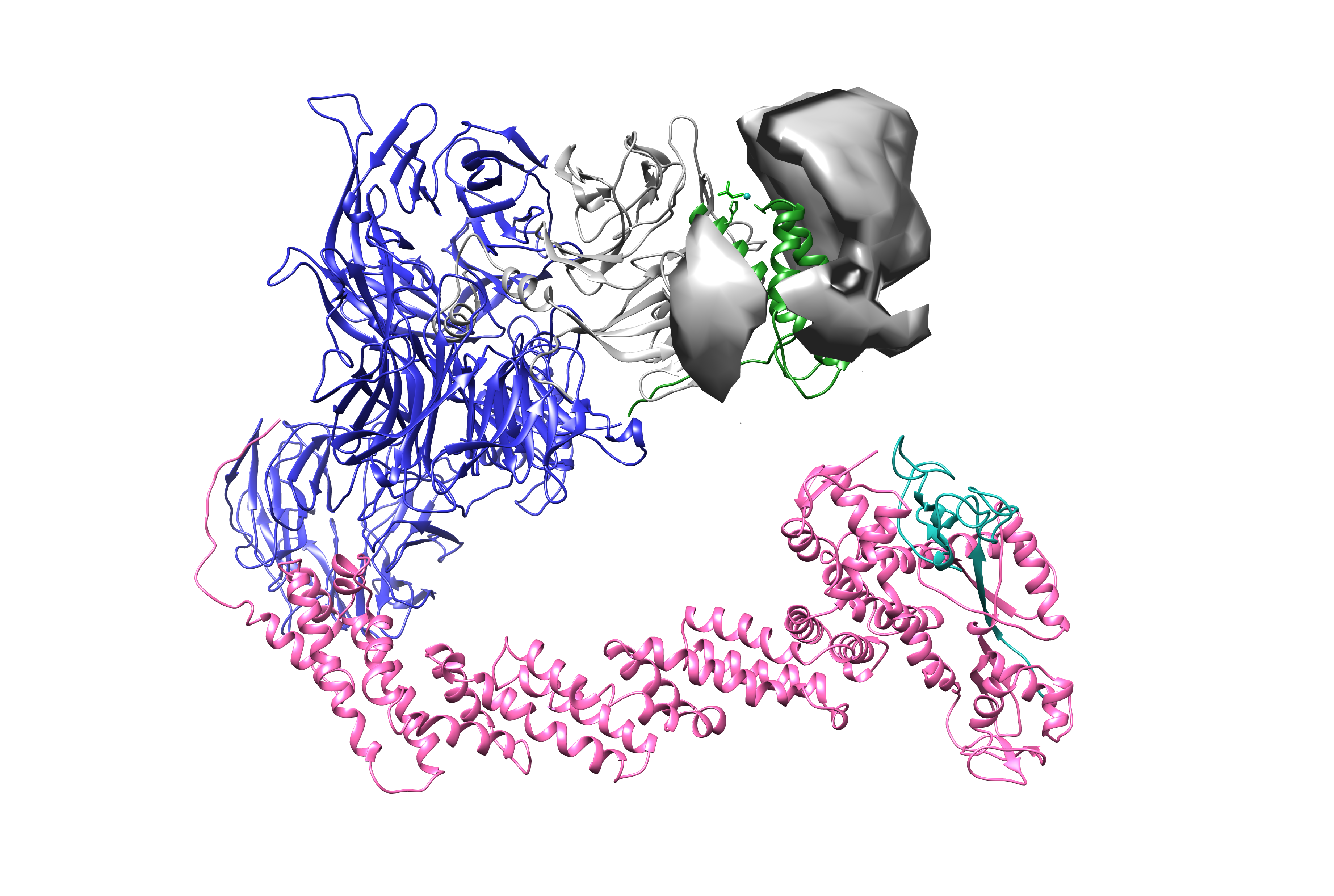
Other modeling approaches
AlphaLink, IMP, Assembline, and HADDOCK provide alternative routes for model building with restraints. They differ in how explicitly they model uncertainty, sampling, scoring, and prior structural information. The correct tool depends on whether the question is exploratory, docking-like, integrative, or prediction-oriented.